Examples

One complete, self-contained example for each algorithm in the library. Every snippet runs as-is: it builds the input, runs the algorithm, inspects the result, and draws it with the matching visualization helper. The # -> comments show the actual output, and each example is followed by the figure it produces.

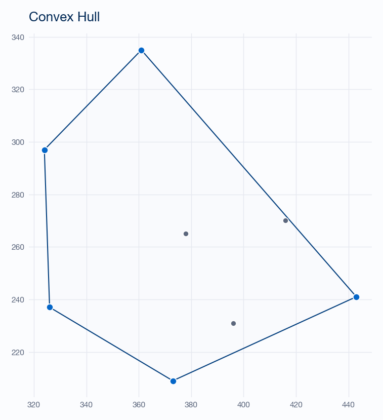
Convex hull

The smallest convex polygon enclosing a set of points (Gift Wrapping / Jarvis march).

from cgeom.algorithms import ConvexHull
from cgeom.visualization import plot_convex_hull

points = [(326, 237), (373, 209), (378, 265), (443, 241),
          (396, 231), (416, 270), (361, 335), (324, 297)]

hull = ConvexHull(points)

hull.convex_hull()   # ordered hull vertices, [[x, y], ...]
hull.get_indexes()   # -> [1, 3, 6, 7, 0]  (indices into `points`)

plot_convex_hull(hull)

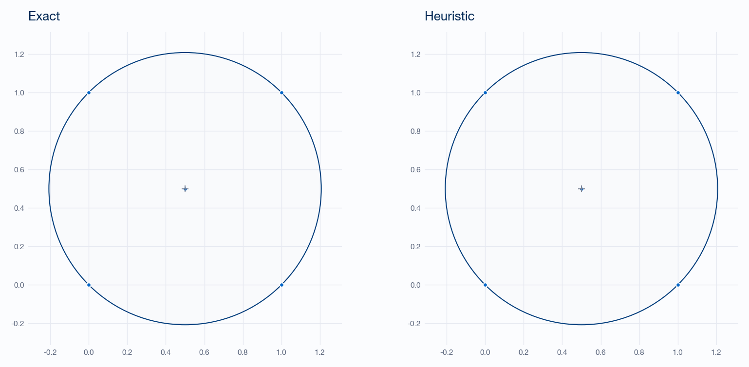
Minimum enclosing circle

The smallest circle that contains every point.

import numpy as np
from cgeom import Circle
from cgeom.algorithms import MinimumCircle
from cgeom.visualization import plot_min_circle

points = [(0, 0), (1, 0), (0, 1), (1, 1), (0.5, 0.5)]

mc = MinimumCircle()
center, radius = mc.minimum_circle(points)   # -> [0.5, 0.5], 0.70710678...

# the raw [[cx, cy], radius] result drops straight into a Circle primitive
circle = Circle(mc.minimum_circle(points))
circle.area                                   # 1.5707...

plot_min_circle(mc, np.array(points))

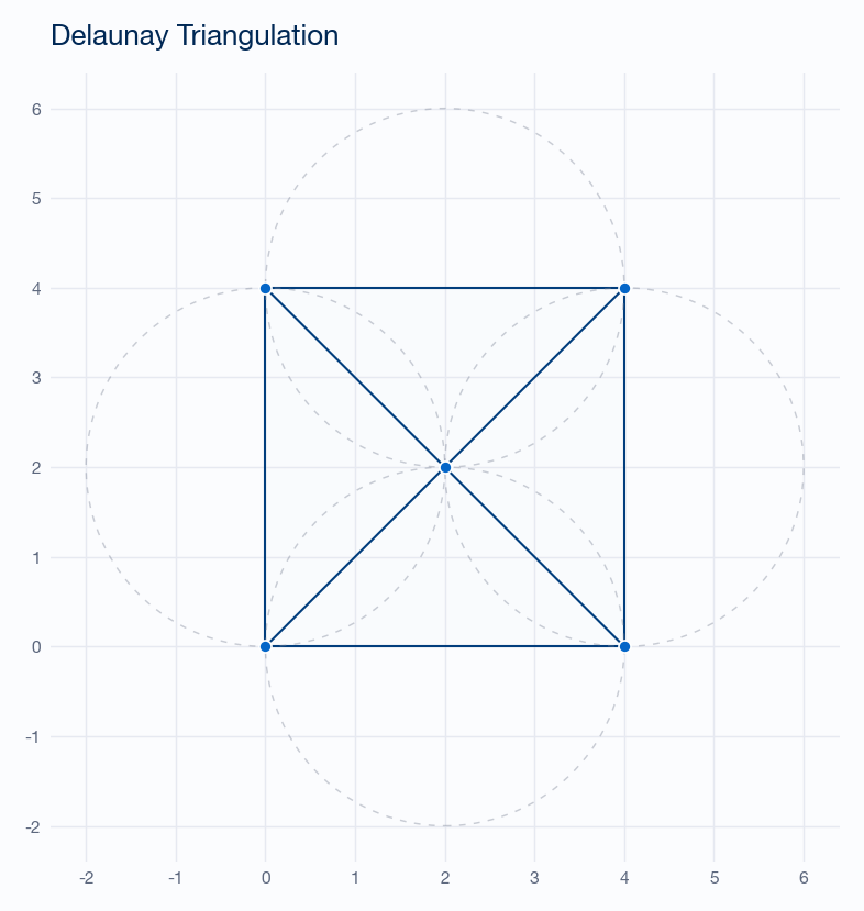
Delaunay triangulation

A triangulation that maximizes the minimum angle — no point lies inside any triangle’s circumcircle.

from cgeom.algorithms import DelaunayTriangulation
from cgeom.visualization import plot_delaunay

points = [(0, 0), (4, 0), (4, 4), (0, 4), (2, 2)]

dt = DelaunayTriangulation(points)

dt.triangulate()             # -> [[0, 1, 4], [0, 3, 4], [1, 2, 4], [2, 3, 4]]
len(dt.get_edges())          # -> 8
len(dt.get_circumcircles())  # -> 4

plot_delaunay(dt, show_circumcircles=True)

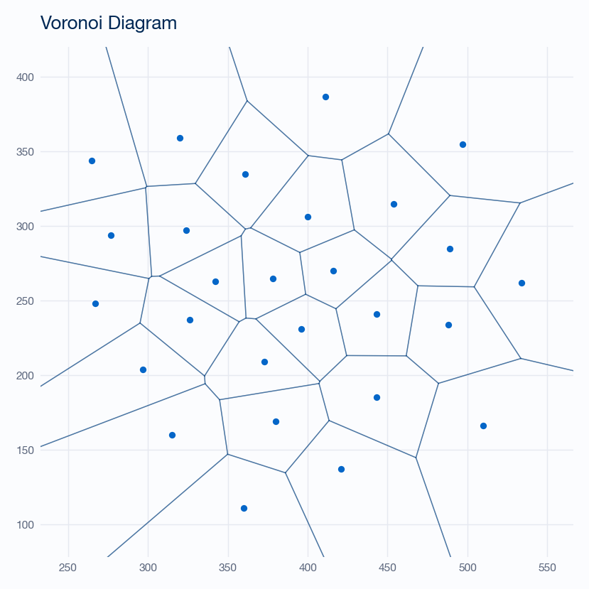
Voronoi diagram

Partitions the plane into cells, one per site, containing everything closest to that site — the dual of the Delaunay triangulation.

import numpy as np
from cgeom.algorithms import VoronoiDiagram
from cgeom.visualization import plot_voronoi

points = np.loadtxt("examples/points1.txt")   # 27 sites

voronoi = VoronoiDiagram(points)
cells = voronoi.build_voronoi_diagram()        # one cell per site
len(cells)                                      # -> 27

plot_voronoi(voronoi, cells)

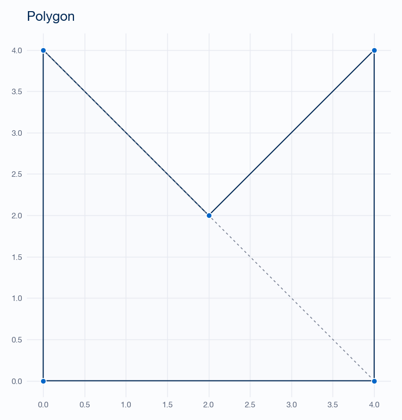
Polygon triangulation

Decomposes a simple polygon into triangles by ear clipping. The polygon is triangulated on construction; the diagonals are available immediately.

from cgeom.algorithms import PolygonTriangulation
from cgeom.visualization import plot_triangulation

# a non-convex pentagon, vertices counter-clockwise
poly = [[0, 0], [4, 0], [4, 4], [2, 2], [0, 4]]

pt = PolygonTriangulation(poly)

pt.diagonals             # the added diagonals, [[[x1, y1], [x2, y2]], ...]
pt.get_diag_vertexes()   # -> [[4, 1], [1, 3]]  (vertex-index pairs)

plot_triangulation(pt)

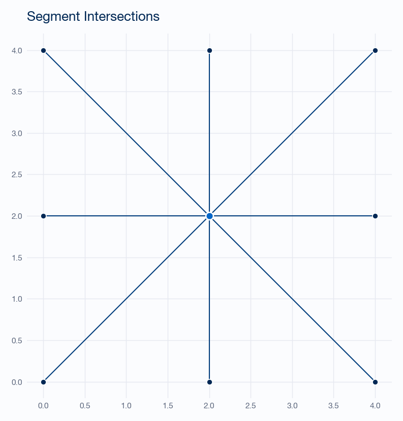
Segment intersection

Reports every pairwise crossing of a set of segments using the Bentley–Ottmann sweep line, with a brute-force method for verification.

from cgeom.algorithms import SegmentIntersection
from cgeom.visualization import plot_intersections

segments = [
    [[0, 0], [4, 4]],   # diagonal /
    [[0, 4], [4, 0]],   # diagonal \
    [[0, 2], [4, 2]],   # horizontal
    [[2, 0], [2, 4]],   # vertical
]

si = SegmentIntersection(segments)

si.find_intersections()              # sweep line      -> [[2.0, 2.0]]
si.find_intersections_brute_force()  # cross-check     -> [[2.0, 2.0]]
si.get_intersection_pairs()          # (i, j, point) for each crossing pair

plot_intersections(si)

See the User guide for the full method-by-method reference, or the API reference for complete signatures. The figures above are regenerated by docs/generate_example_figures.py.